How quickly have machines always been taking our jobs?
High-level takeaways from 150+ years of occupational data

When I first came across this chart from the Fed several years ago, I became rather obsessed with the Census data behind it. How cool to be able to able to get a quick visual of how much jobs have changed over such a long period of time!
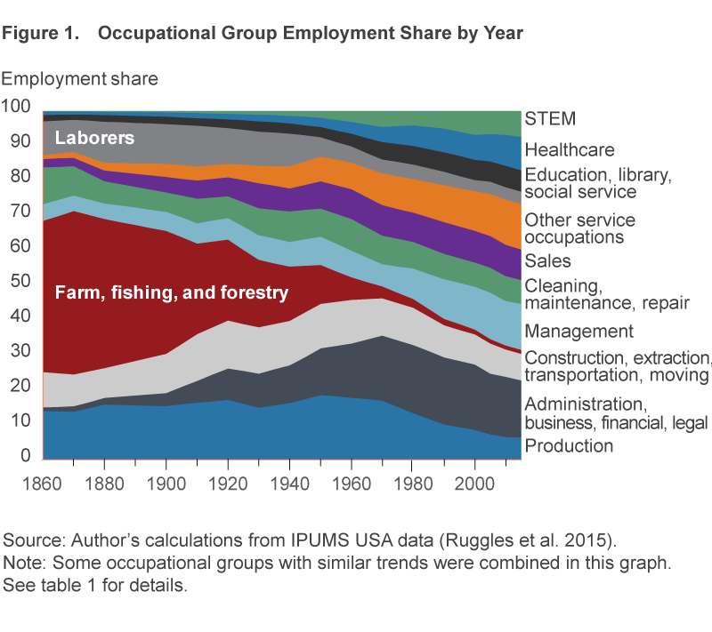
The huge decline in agriculture and production jobs, and the emergence of STEM work from almost nothing, all technology-driven, is immediately visible. But aside from these major changes, this is quite a noisy chart. How can it tell us how normal or unprecedented the evolution of jobs in the recent past has been?
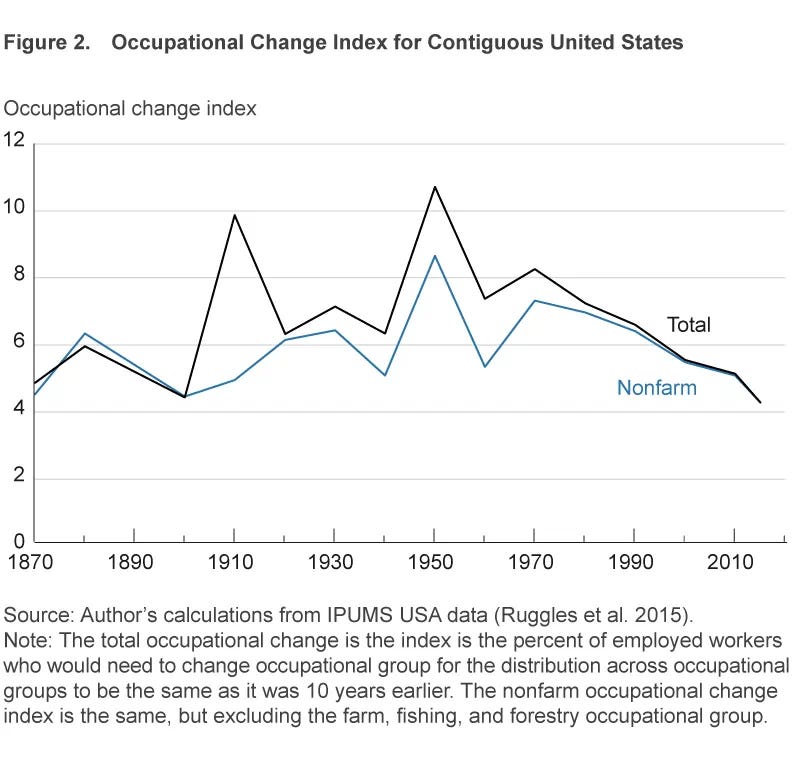
This second figure from the original Fed analysis, which measures how much the distribution of jobs in each decade varied from the previous one, helps answer that question. But the results surprised me. How could it be that jobs changed less in the 2010s than any other previous decade?
There were certainly some flaws and oversimplifications in the methodology. For example, it only measures changes across high-level categories. While it might capture major shifts like workers switching from farms to factories, or from factories to driving for Uber, it doesn’t count shifts between more similar lines of work, like going from data entry to customer service work.
A few years ago, I took a first crack at measuring the changes at this more detailed level, and visualized what they looked like in each decade up to 2019. It roughly confirmed what the Fed also concluded: not as many people switching occupations as back in the day.
But I was still unsatisfied. The definitions of jobs have shifted over time, and this is poorly accounted for in the original analysis. There were some significant realignments in 1970, 1980, and 2000. Could these make the rates of change observed in the past seem greater than they actually were?
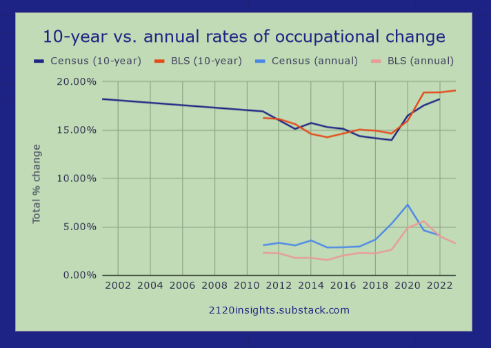
After discovering tables like this from the Census, I found a way to largely control for this factor too.1 And the story remains similar, whether using Census (individually-reported) or BLS (employer-reported) data2. That is, until 2020. Let’s zoom in on the past three plus decades since 1990, and up to 2023.
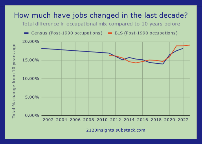
Unsurprisingly, the pandemic and its aftermath changed a lot. The 2010-2020 change of roughly 16% of the workforce turning over is the most observed since at least 2003-2013. But rather than people returning to the same occupations after the pandemic, change continued to be above average through 2023, bringing the 10-year rate of change past its previous high in the 1990s!
It’s important to note that no single year was more significant than 2020, which saw about as much change as we typically see over 3-5 years3. But 2021, 2022, and 2023 were all above average individually, which continues to bring that 10-year moving average up. Even 2023 saw more than twice as much change as 2015, which was only a little less than where we were at in the depths of the Great Recession.
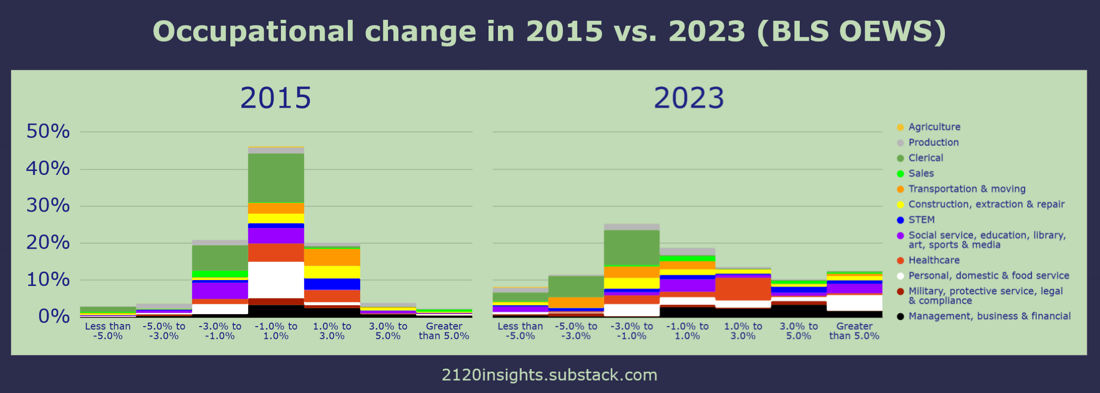
Comparing some of these key individual years, we can see how strikingly different they are. Even though there was a significant decline in clerical jobs in both 2015 and 2023, these losses have accelerated, and many other types of jobs can also be seen on the extreme ends of either faster growth or decline.
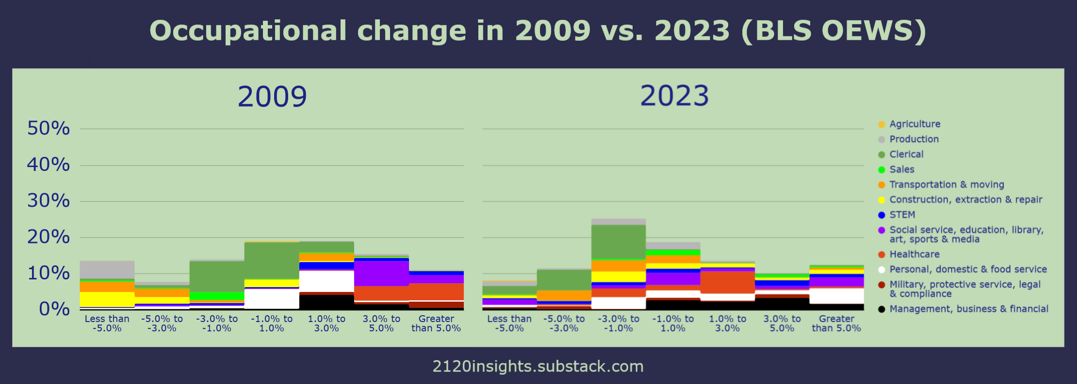
While the overall rate of change in 2009 was similar to 2023, there is a much clearer breakout by sector with big recession-era declines in blue-collar construction, production, and transportation jobs, and relative increases in healthcare and education. It’s also important to note that these figures are relative to employment overall, so even the “average” occupations toward the middle still saw significant losses in 2009. The reverse was true for the growing labor force of 2023.
The shift in work during the 2020s appears to be a lot more complex than what happened during the Great Recession. There is a lot more that we could dive into here, but let’s zoom back out and think of how this overall rate of change compares to history.
The big picture
We can make reasonable comparisons to more historical decades by using a broader standard for the definitions of each occupation that holds up better over time. Rather than measure the total amount of change across 406 occupations that are tracked from 2000 onward (and for Census data, backdated to 1990), we can use 246 more general occupations that still cover the full range of employment and backdate to 1970 while still controlling for the smaller re-definitions that have occurred since then.

Similar to the Fed analysis, we see even more change in the 1970s and 80s. Naturally, because we are tracking against the 246 broader occupations, there is less variance overall than if we measured the change across the 406 narrower occupations after 1990-2000.
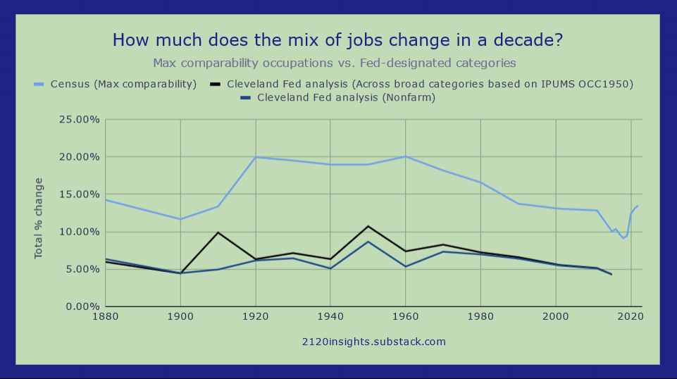
But we can use an even broader standard of 133 more general occupations that go all the way back to 18704:

From this, we see that even the 1970s and 80s are at the back end of a wave of significant changes in the types of jobs that Americans worked. The 2000-2010s were unusually stable decades in terms of changes in the occupational mix, and the economy of the 1910s-1960s was about twice as dynamic in this regard!
Comparing this analysis with the original Fed one, we can see that in most years, changes in occupations within categories (e.g. from office clerks to secretaries) are usually much more common than changes across categories (e.g. farmers to truck drivers)— this difference is represented by the gap between the black line and the light blue one above vs. the difference between the black line and zero.
Excepting the Great Depression, 1910 through 1970 was an economically dynamic period. Meanwhile, the de-industrialization of the 1970s and 80s happened amidst a decline in the rate of occupational change, and the economic recovery of the 2010s happened at record-low rates of occupational change. There doesn’t seem to be a clear relationship between changes in the types of jobs and economic growth. What else are we missing?
Deeper questions
So far, our metric for occupational change has just measured how different a current distribution of jobs is compared to 10 years before. This is a good high-level overview that compares nicely with metrics used by the Fed analysis and the BLS5, but it misses a few things. For example, it doesn’t capture how much the changes were concentrated in a few specific jobs vs. spread out across the wider economy. This is a really important consideration: some of the steepest declines in employment in particular trades in the past have been technology-driven. As we anticipate how big of an impact AI and robots might have on our future job market, it can be helpful to see at a high level how often these sharp declines have occurred in the past.
Using a weighted standard deviation of job growth rates can help us see this, as the extremes factor more heavily. To ensure that significantly declining occupations are considered similarly to significantly growing ones, we should use annualized growth rates rather than 10-year ones6.

Tracking this shows that the 1910s and 1950s saw more extremes than the other years between 1910 and 1970. Both of these decades were driven by a notable exodus from agriculture. In the 1910s, it was farm laborers, but the 1950s saw an even sharper decrease in both laborers and landowning farmers.

Subtracting the average overall amount of change from the standard deviation can get us a measure that is similar to kurtosis and helps us highlight some other decades that saw unusually sharp changes relative to the overall average.
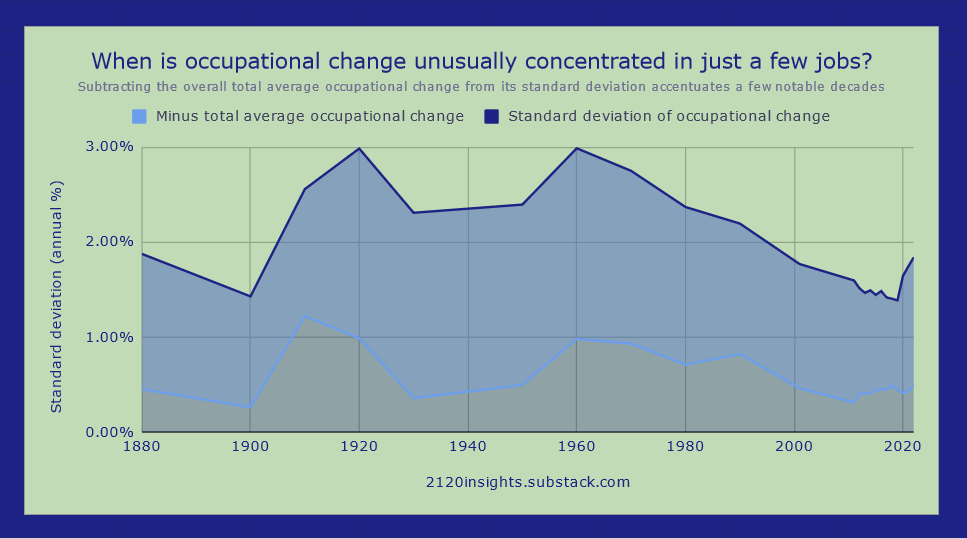
The 1910s and 1950s are still notable here, but it is the 1900s which really stand out in this case. When we look at the distribution of change in the 1900s, we see a relative decline in the percentage of the workforce who were landowning (or tenant) farmers. But in terms of absolute numbers, there were still more farmers in 1910 than there were in 1900! Employment in this area didn’t actually start declining until the 1920s (with a decline in farm workers preceding it in the 1910s).

This is because the wave of immigration and urbanization in this decade made growth in most other occupations dwarf the growth in farming.

So this historic example of a (relative) decline in farming isn’t something that should worry us too much in anticipating scenarios of job-replacing robots. But there is another decade highlighted by this metric that warrants more of our attention: the 1980s.
A key indicator of robots taking our jobs
The significant loss of manufacturing jobs was one of the defining features of the 1980s job market. While there was certainly growth in other occupations that offset this to some degree, increases in employment elsewhere were more tepid. This is quite a different scenario from all other decades from 1910 to 1980 where strong growth is some sectors was able to provide work for those leaving agriculture or other manual labor occupations.

There is one more metric which we can use to estimate the degree to which there was a balance between people being “pulled” into growing occupations vs. “pushed” away from declining ones: the weighted skewness7.
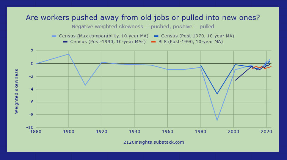
A positive metric here means the distribution is more heavily weighted towards quickly growing occupations; a negative one means it is more weighted toward quickly declining ones. The 1980s immediately jump out as the most negative decade by a long shot.
This chart tells an incredible story though: the labor market does tend to “push” workers from existing jobs rather than “pulling” them into new ones overall, but in some decades, the effect is more pronounced than others. Only in a few decades was growth in some occupations more concentrated in declines elsewhere. The 2020s labor market is one of those rare exceptions, depending on how you measure it8.
The implications of occupational change on technological development and politics
I think the experience of de-industrialization and its associated job loss in the 1980s and early 90s scarred us in America, and still has a deep-seated influence on our political rhetoric and priorities in the 2020s. Even with unemployment near record lows, and indicators like the ones above suggesting that the job market is being more driven by growing new fields rather than jobs being automated or outsourced away from declining ones, there is still a pessimistic outlook that colors the American perception of AI. These sentiments are different in other parts of the world that had a very different experience with technological advancements and occupational change over the past few decades:

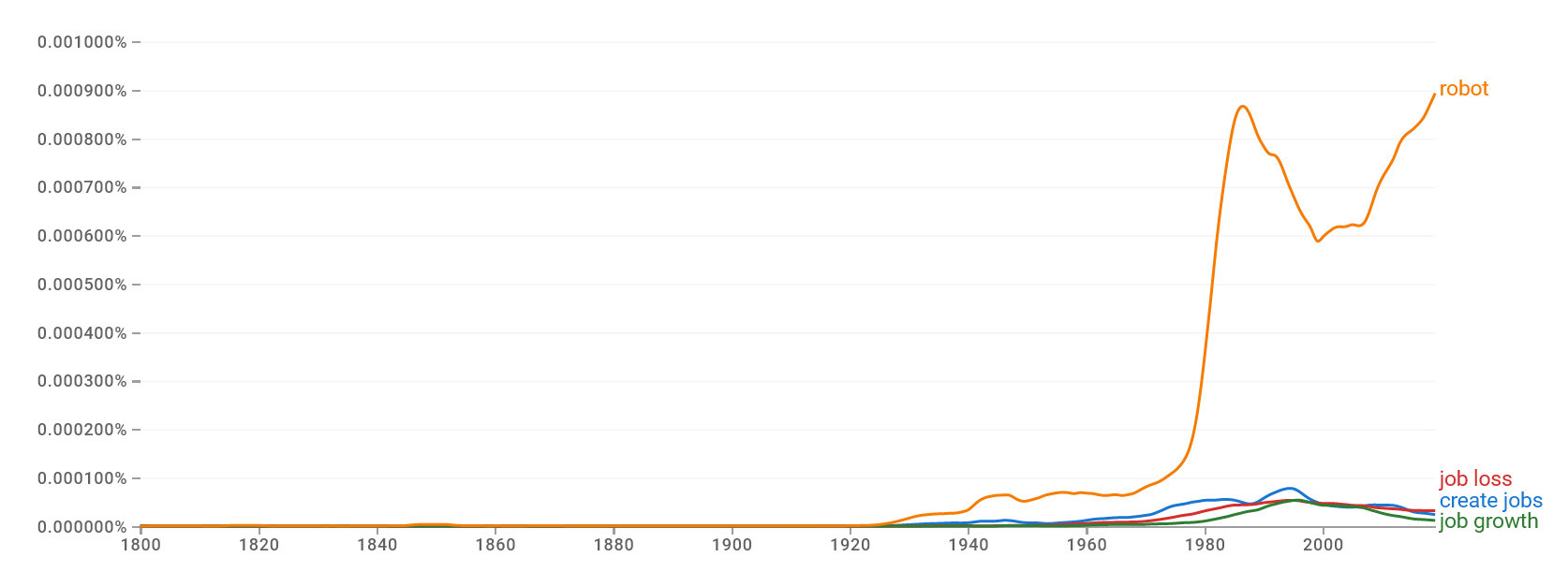
Mentions in the literature of “job loss”, job creation, and related terms as measured by Google’s ngram viewer provide another interesting way to measure just how much of an impact the experience of job losses in the 80s had on public discourse in the English-speaking world.
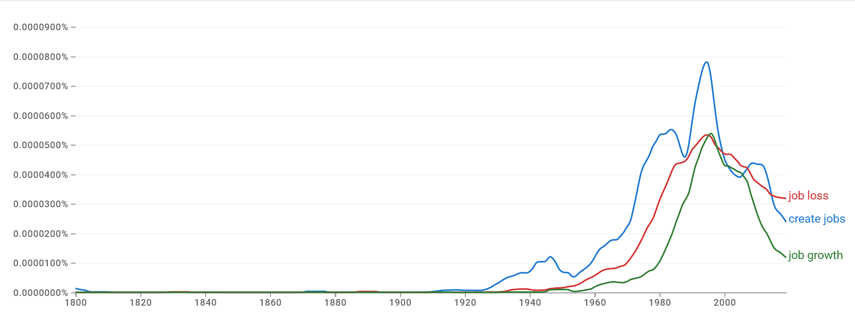
Until the 2010s, mentions of these terms rose and fell with mentions of robots.
These fears are still very much in the public consciousness. And this makes sense. The median voter in the US came of age around 1990, and a second wave of job loss in manufacturing (and also construction) during the Great Recession was a near-repeat of this experience that many in their thirties and forties remember too.

What the indicators say now
New developments in AI and robotics, among many other factors, could accelerate layoffs again in the future. But when would we know if this actually happening?
While the above metrics of occupational change are based on Census ACS and BLS OEWS data that are some of the least timely indicators (coming out almost a year or more after initial surveys), there are ways to catch these changes much earlier. An unexpected rise in weekly unemployment claims from states might direct more attention to the next monthly Current Employment Statistics (CES) and Current Population Survey (CPS) reports from employers and individuals respectively. Further confirmation of any observations from the monthly reports could be confirmed about about a month later when results from the Job Openings and Labor Turnover Survey (JOLTS) are released. And if fewer job opening are recorded, the ratio of unemployed per job opening from this report can sometimes be a leading indicator of changes to come.

As of this writing, JOLTS still indicates that there are more job openings than unemployed workers, but the slight upward trend in initial unemployment claims means this ratio might rise in an unfavorable direction when April 2024 data is released in the first week of June. If this trend continues, I will plan to do a special analysis into what this change in employment looks like, and if it shows any similarities to previous technology-driven layoffs.
Where the numbers disagree
As I have taken a closer look at the long-term trends and puzzled over how they connect to the latest numbers, I’ve encountered a few challenges in reconciling differences between the various surveys. This probably merits some more in-depth explanation in a later piece, but a few observations for now:
While the more comprehensive annual surveys break down employment by detailed occupation (as well as detailed industry), the CES survey only reports by detailed industry, and JOLTS only reports a breakout of high-level industry.
This is fine for occupations are so concentrated in particular industries (e.g. software engineers in Computing Infrastructure Providers, Data Processing, Web Hosting, and Related Services) that a significant change in industry employment can also suggest a change in demand for a particular skillset.
However, many jobs that might be under threat of being automated by AI (e.g. customer service representatives) are so spread out across various industries that it is hard to follow their trajectory month-to-month.9
The more detailed and timely BLS employer-reported surveys like the CES don’t capture some types of self-employed and “gig” workers that are counted by Census surveys like the ACS and CPS. However, these can often be some of the fastest-growing jobs.10
With all this in mind, I hope to model out what the employment numbers might look like during a realistic rollout of self-driving cars, humanoid robots, or more autonomous virtual agents. Better understanding the rates of historic changes, and the context around them (including the ambiguities that are likely to arise) I think are critical for making projections that capture the complexities of the real world and aren’t overly reductive. One of the biggest questions that the 2020s and 2030s may put to the test is if the rate of automation might again exceed the economy’s capacity for adding new jobs. In their report from the spring of 2023, researchers from Goldman Sachs put this at about 0.5% per year, based on this paper from economists Daron Acemoglu and Paul Restrepo.

If technological displacement begins to exceed 0.5% of the workforce per year, will that intensify efforts to bring about a shorter workweek, or cause a “race to the bottom” for wages? Or have we entered a new phase of economic development where new jobs are being created fast enough to offset any displacements that might occur?
Predicting the new jobs of the future
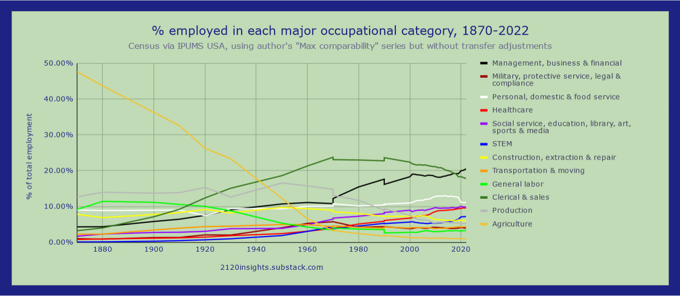
I often wonder how much predicting the jobs of today would have been possible in the past. I made a chart similar to the original Fed one, but de-stacked it to more clearly see the trends in each occupational category.

One trend that seems quite apparent to me is the growth of the “Management, business & financial” category. As technology becomes more powerful, does this mean that managers are more empowered to do work themselves?
It took me many months to clean up the data behind this chart enough to be more comparable back to 1870.11 The depth and breadth of it go far beyond the high-level CPS occupational figures available in FRED— being able to easily drill down to each occupation individually can allow one can see details of professions that declined dramatically as examples of how future technological displacement might play out. The complexity of the significant changes in occupations in 2023 wouldn’t be visible any other way. There are so many stories behind this data that I look forward to sharing over the coming months!
The way in which occupations have been reclassified over time is quite confusing, so it’s best to give a specific example with a visual:
“Insurance and other financial products agents and brokers” is an occupation that has been tracked consistently over time, but some workers classified as “General office and administrative support workers” in most other years have occasionally been included as well. A Sankey diagram can be one of the best ways to visualize the impact of these changes in definition:

As we can see, the definition of this occupation in 1970 is much more broadly inclusive, but only temporarily. The growth in employment between 1960 and 1970 is almost entirely due to the change of definition, which is adjusted again in 1980 to exclude many of the workers who were counted in 1970 but not in 1960. To reduce this error, my estimates of employment in occupations in 1970 are based on the Census tables referred to here which estimate how many workers in 1970 would have been in each 1980 occupation, and how many workers in 1960 would have been in each 1970 occupation. Carrying the 1960 ratios forward and comparing them with the 1970 employment estimates based on 1980 occupations ends up matching up nicely in this case.
Note that the jump in the 3rd stage just shows the increase in employment in this field between 1980 and 1990 when no change in definition occurred.
Also note that these aren’t the actual Census classifications, but a “max comparability” classification that I developed specifically to reduce the amount of error occurring across more narrowly defined Census occupations (which I have combined in many cases where the evidence of these shifts in definition have supported it— I address this in more detail in another footnote below).
The BLS does track occupations at a more granular level than the Census, but I have controlled for that by creating a new list of 406 broader occupations that are common and consistently tracked by both systems starting in 2000. I refer to these as “Post-1990” occupations. These crosswalks provided by the Census were essential for determining what the lowest common denominator was between Census OCCs and BLS SOCs, but some manual additions were needed where the crosswalks are incomplete. This is particularly true of occupations that only existed temporarily, or that hadn’t yet been defined by the BLS in 2018. The lowest common denominator “Post-1990” occupations are in many cases synonymous with the OCC2010 occupations provided by IPUMS, but with 4 exceptions:
A few OCC2010 occupations were not consistently tracked over the post-2000 period, either in the Census or their crosswalked BLS equivalents. No, there wasn’t a huge drop in elementary and middle school teachers in 2019. It just appears that the occupation was redefined in the Census, so I combined these four occupations into a single “Post-1990” occupation of “Teachers, pre-k-12”.

On the flipside, a few OCC2010 occupations whose Census OCC codes (and their BLS OEWS equivalents) could be tracked consistently back to 1990-2000. In these cases, I split them out as separately (e.g. OCC 1800 “Economists and market researchers”).
A handful of Census OCC codes were assigned to an OCC2010 occupation that I disagreed with. For example, the supervisory nature of OCC 4000 “Chefs and Head Cooks” seems to make it a better fit for OCC2010 4010 “First-line supervisors of food preparation and serving workers” than classified alongside the line employee “Cooks” of OCC 4020.
Some minor changes in definitions of these 406 occupations have occurred since 2000.
Tables like E1-E3 from this Census page detail some changes in 2018 as “occupation conversion rates”.
Where these changes cross the boundaries of the 406 Post-1990 occupations that I have defined, I listed them on a separate table in my internal spreadsheet that calculates the totals for each occupation. In some cases, I combined the occupations into a single Post-1990 designation to minimize the number of adjustments made.
The BLS does not provide equivalent tables documenting changes in definitions. Where there were unusual unexplained jumps or declines in numbers, I interpolated an estimate of the possible number of workers affected by the change based on the combined growth of the two occupations where I suspected a change in definition happened. But in general, these sorts of adjustments were less common for BLS data compared to Census data.
Where a change in definition occurred (or may have occurred), the adjustment usually has to be made in all years going forward. My adjusted totals calculate what employment might continue to be in a particular occupation had the definition remained constant since 1990-2000.
However, making such estimates requires making a crude assumption that in the years following the change in definition, growth in the number of workers whose occupations were redefined remained consistent with employment growth overall. This approach may be fine for a decade or two, but I may need to make further adjustments to it in the future.
A possible change in methodology might involve using more sophisticated predictive models like the ones outlined here to determine how many workers historically classified as a particular occupation might have fit under a new, more modern definition. Recent advances in AI might be able to augment this approach.

Each individual year’s rate of change is much higher than 1/10th of the 10-year rate. Individual years are “noisier” in this way than decades because some occupations see resurgences after losing ground and vice versa.
The 2015 Fed analysis of occupational change cited above uses 1950 occupational categories (OCC1950). However, some of these completely disappear after 1970 or afterwards due to the reclassifications of 1970 and 1980.
To minimize these losses over long time horizons, I created three series of inter-related occupational classification systems:
A child “Post-1990” series (explained in this footnote above).
A parent “1970 broad” series
A grandparent “Max comparability” series
The parent and grandparent “1970 broad” and “Max comparability” series combine some of their child occupations such that there is either a 1:1 or 1:many relationship between parent and child. This allows for the lineage of newer “child” occupations to be more clearly defined. Looking at a child series allows for a more detailed analysis from either 1970 or 1990 going forward, while looking at a parent series allows for a rough comparison of broader occupations over a longer period of time in a way that can be adjusted to be consistent across the 1970, 1980 and 2000 reclassifications. The broadest “Max comparability” series allows for rough comparability of occupations in Census data going all the way back to 1870.
While the Post-1990 series is roughly based on the OCC2010 occupations from IPUMS, the “Max comparability” series is based on their OCC1950 occupations, with similar caveats for pre-1970 data:
Many OCC1950 occupations, in particular ones that later disappeared, are combined into more general occupations. And unlike the relationship between my “Post-1990” categories and OCC2010, no “Max comparability” occupations are defined more narrowly than the OCC1950(s) they are associated with.
There are also a few occupations whose OCC1950 designations in 1970 I disagreed with and reassigned to a different OCC1950, but there are only 3 of these and all of them were very small.
Between using this table to make estimates of employment in 1970 by OCC1950 consistent with how occupations were defined in 1960 (assuming the proportion of reassigned workers remained the same in 1970), and using this table to bring accurate OCC2010 estimates of employment back to 1990, getting an accurate count of employment from 1870-1970 and from 1990-2022 was relatively straightforward. Building the intermediate “1970 broad” series that bridges these two systems such that there is only one parent for each child occupation was the most difficult task.
There is an intermediate OCC1990 series available that some researchers use to bridge this gap. However, this series has its limitations:
Some OCC1990s effectively have multiple OCC1950 parents, which makes comparability across 1970 challenging unless some of the individual OCCs under the OCC1990 are changed, or the OCC1950 is broadened into a “Max comparability” category (I have taken both approaches).
Some OCC1990s do actually offer more detail than the OCC2010 occupations that succeed them (particularly production ones). However, if we want to have a series that we can reliably compare from 1970 going forward, the intermediate “1970 broad” series must be at least as broad as the “Post-1990” series (which itself is mostly based on the separate OCC2010 series).
The complexity of the adjustments I made to achieve these three more comparable series are hard to explain in words alone. Here are a few Sankey diagrams that explain the problem for one of the occupations that was most difficult to track consistently over time, and my solution:
Note that in the following charts, the dates refer to the original OCC years; 1960 and 1970 figures represent estimates of 1970 employment across the two different systems, and 1980 and 2000 figures represent similar estimates of 1990 employment.
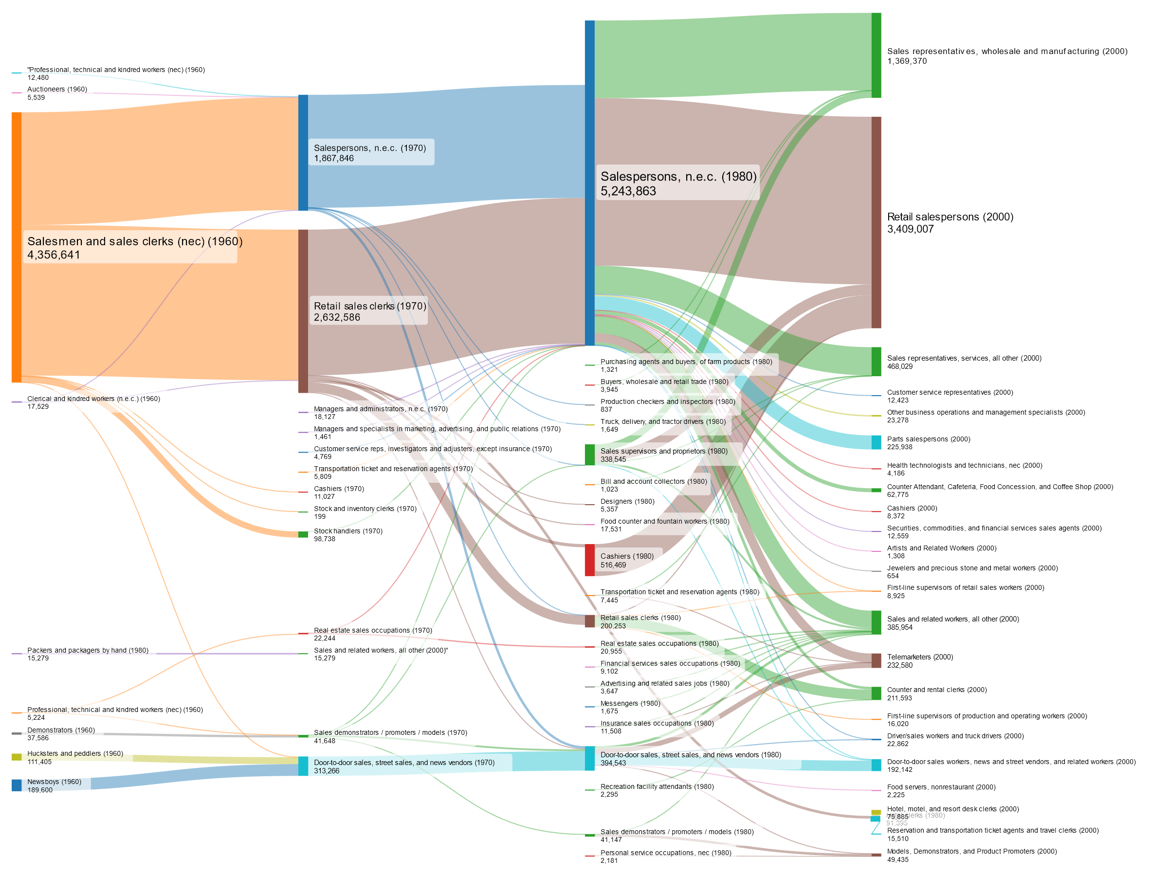
Here are the original Census occupations (OCCs) for each year 1960-2000 and transfers between them for all workers counted in my max comparability occupation “Retail and other sales workers”

What a mess! Here’s how these occupations look when put into their broader OCC1950, OCC1990, and OCC2010 categories:
Noticeably cleaner, but there is still a lot of inconsistency. By reassigning a few of the child OCCs to OCC1990s that are a better fit, we can further reduce that error across years:

However, my proposed system of “Max comparability”, “1970 broad”, and “Post-1990” is even cleaner: we can see a clear generational progression here from a general “Retail and other sales workers” category with some specified sales representatives broken out in 1970, and other more detailed sales occupations broken out in 1990-2000.
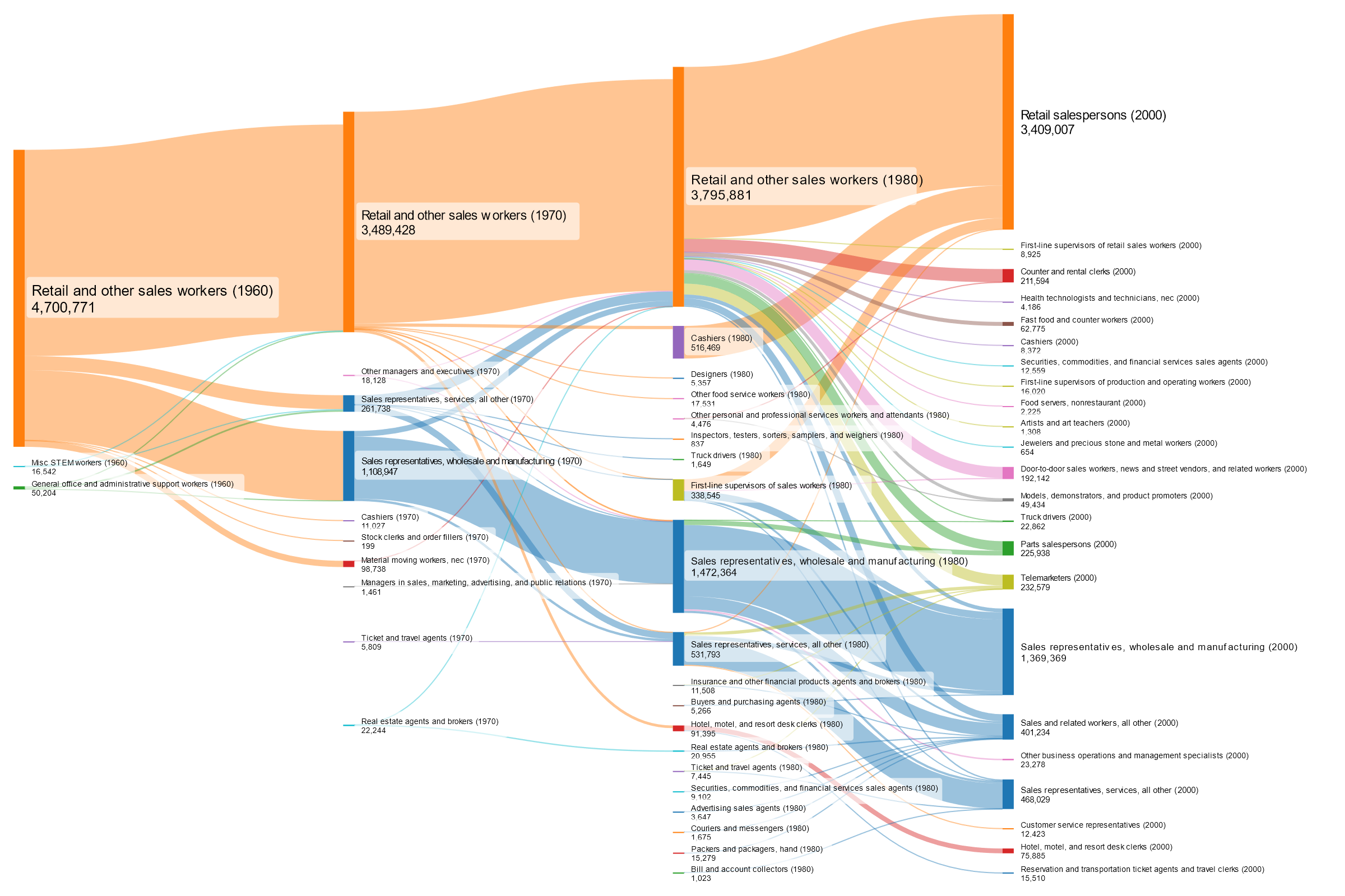
Some error still exists, but it is small enough to control for it in my other charts in two different ways.
The first approach is to show values for both the previous and new definitions of an occupation for each year that a redefinition occurs:
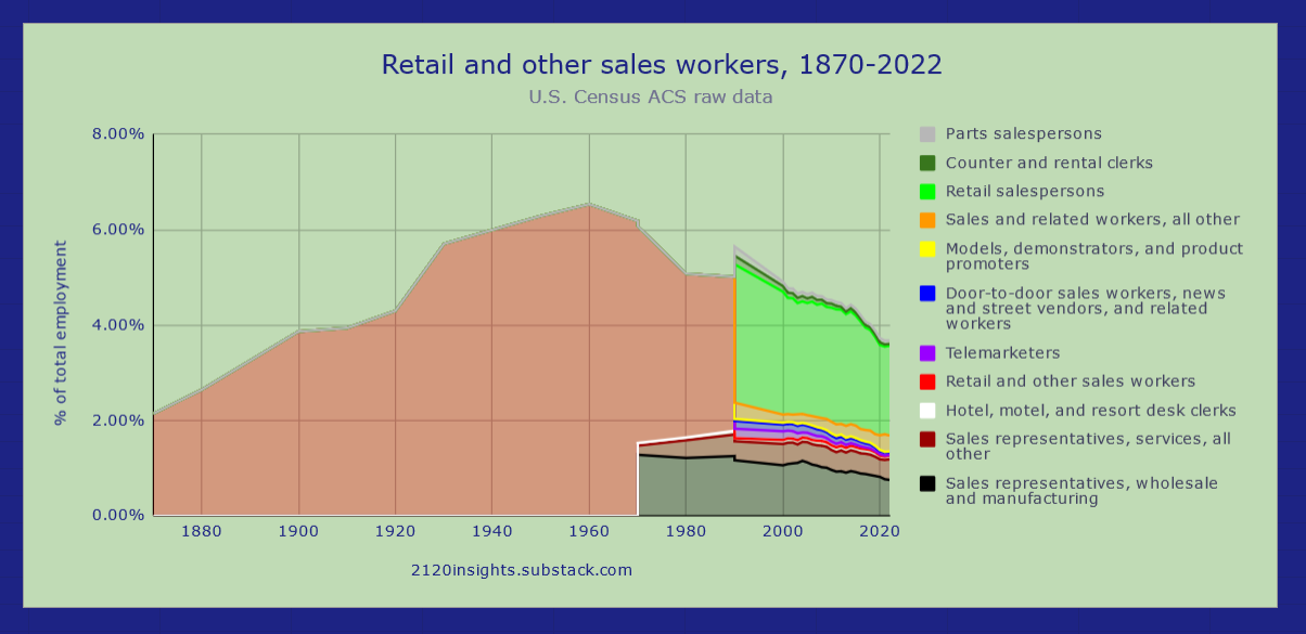
While this chart doesn’t show the details of what other occupations some individuals were reassigned from and to in the key years, it does show conspicuous drops that make it clear that a reclassification happened. At the same time, these drops are small enough that we could conceivably imagine how many people would today be counted in the earlier definition of an occupation by assuming* that the (small) difference has grown proportionally with overall employment.
*Note that this is an assumption we have to be most careful about in occupations that have seen significant decline, somewhat careful in occupations that have seen significant growth, but can tolerate more error if the occupation in question has grown roughly in proportion with employment.
If we want to make this assumption and imagine how many workers today might have been counted in the pre-1970 bundle of old occupations represented by the “Max comparability” occupation, we get a simple chart like this:

Designing these three series took a considerable amount of time and judgement, but the resulting occupations are significantly more comparable over time than the existing OCC1950, OCC1990, and OCC2010 designations. Here is how much error was reduced using max comparability series across 1960-70, and using 1970 broad series across 1970-80 and 1990-2000 relative to the OCC1990 occupations:

Across each of these key years, between 16 and 26% of workers had their occupations reclassified by the Census in a significant enough way to shift them into another OCC1990 occupation. I was able to slightly reduce this by changing which OCC1990 70 different individual Census occupation codes were assigned to, and more significantly reduce the error by combining multiple OCC1990 occupations into broader “Max comparability” and “1970 broad” ones. These approached occasionally reintroduced some error (mostly from there being a minority of workers who were correctly designated in their original OCC1990, but outweighed by a majority who were not). Nevertheless, total error was reduced by nearly 80% across the 1960-70 transition, and by roughly 50% across 1970-80 and 1990-2000.
When considering these broader definitions for some occupations, there are both inflows and outflows that roughly balance each other out. For example, the 1970 broad occupation “Medical assistants and other healthcare support occupations, nec” sees many workers who had some practitioner duties moved into other practitioner-specific healthcare occupations (e.g. “Licensed practical and vocational nurses”), but this outflow is roughly balanced out by some clerical and technical workers such as “Cashiers” and “Other health technologists and technicians” moving into the new 2000 classification.
If we want to track salaries and hours, a 16% outflow offset by a 20% inflow is still a significant change that one should be cautious about making assumptions about. But if we are just adjusting for the overall number of workers, a 4% change is easy to control for. Overall, the distribution of net transfer error across 1960-1980 (combining the 1960-70 and 70-80 classification changes) is under 20% for most max comparability occupations.
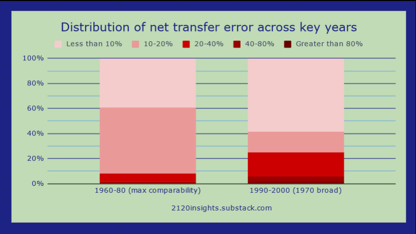
The reclassification of 1990-2000 cut some occupations a little deeper, with nearly 25% of workers in occupations whose definitions shifted by 20% or more on net. However, there is less time to account for after 1990, so more error can be tolerated. The occupations that I allowed to remain distinct even with a larger amount of transfer error tended to be ones where employment growth was roughly in line with overall employment growth, with a few exceptions. However, these designations may need to be revisited should employment shift significantly in the future. A better approach at that point may be to use AI to analyze how many historic occupations would have fit into a more modern classification rather than trying to imagine how many people in today’s workforce would have fit into 1950, 1970, or 1990 occupational designations.
It’s worth noting that the BLS metric for occupational change is slightly different from the approach used by the Fed and my own analysis. The formula I use is as follows:

Essentially, I take the total difference between the initial and final year employment for each occupation, and divide it by total final year employment. The Fed analysis takes this approach as well, but only measures major category differences rather than individual occupation changes.
However, the BLS effectively takes how much each occupation has changed as a percentage of overall employment, and sums that up to a total that ends up being numerically similar to my formula for calculating the total amount of occupational change, but the units are not technically expressible since the denominators are slightly different:

It’s also worth noting that my approach includes all occupations, but only at the broader “Post-1990” level. I make some interpolated estimates (detailed in this footnote above) where changes in the definition of one of these broader occupations likely occurred. Meanwhile, the BLS measure of occupational change is calculated using the more detailed SOCs, but excludes SOCs that merged together in later years or were otherwise transformed such that the changes have a many-to-many relationship.
Effectively, the broadness of my post-1990 classification system reduces the overall occupational change estimate a bit. But the exclusions reduce the BLS’ overall estimate as well, resulting in similar numbers of 18.9% and 17.8 for 2012-2022 (the “sum of absolute differences” for the Naïve model effectively measures the total change in occupations between 2012 and 2022).
If we were to use 10-year growth rates rather than annual ones, growing occupations would be weighted much more heavily than declining ones. Over 10 years, an occupation growing at 7% per year would have roughly doubled, giving it a weight of 100%. An occupation declining at 7% per year would be halved over 10 years, but it’s weight of -50% would only be half as strong. This is not what we want if we want to highlight fast-declining occupations so we can better look out for them in the future!
ChatGPT really helped me learn how to measure weighted skewness. Knowing that it has a tendency to sometimes make things up, I spent a bit more time validating what it told me than I would if I read the same content in a textbook, but I think this exercise helped me learn the concept even better than I might have otherwise. Here is it’s explanation, which checks out as far as I am aware:
Calculating the weighted skewness of a distribution in Google Sheets requires a bit more effort than calculating the basic skewness, as Google Sheets does not provide a direct function for weighted skewness. However, you can use a combination of formulas and steps to achieve this. Weighted skewness takes into account the frequency or weight of each value in the dataset, providing a measure that's more representative of the distribution when each observation doesn't contribute equally.
Here's how you can calculate the weighted skewness:
Step 1: Prepare Your Data
Assume your data is in two columns: Values (A) and Weights (B), starting from row 2 to n.
Step 2: Calculate Necessary Statistics
Weighted Mean:
Formula:

In Google Sheets, if your data is in
A2:A, and weights are inB2:B, you can calculate the weighted mean in a cell with:
=SUMPRODUCT(A2:A, B2:B) / SUM(B2:B)Weighted Variance:
For each value, calculate the squared difference from the weighted mean, multiply by its weight, sum all these products, and divide by the sum of weights.
Formula:

This needs to be done with a combination of
SUMPRODUCTfor the numerator andSUMfor the denominator.
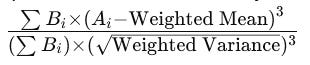
Weighted Skewness Formula:
Skewness is a bit more complex to calculate directly in Google Sheets due to its formula:

You'll calculate the numerator as a sumproduct of the weights and the cubed differences from the mean, and the denominator as the sum of the weights times the cubed root of the weighted variance.


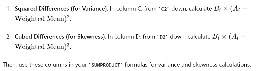
Step 3: Implementing Weighted Skewness
Due to Google Sheets' limitations, you'll need to use helper columns to calculate the squared and cubed differences from the weighted mean, multiplied by their weights, for the variance and skewness calculations, respectively.
Note:
Directly implementing these calculations in Google Sheets, especially the weighted skewness part, will require creating and managing several intermediate calculations and potentially large helper columns, which can be cumbersome for very large datasets.
If your dataset is sizable or you require more sophisticated statistical analysis frequently, consider using statistical software or programming languages like R or Python, which offer more direct and powerful functions for such computations.
This metric is more positively skewed in the Census moving average (MA) due to some shifts in occupational definitions in 2018 that my methodology hasn’t fully accounted for. When measured annually, weighted skewness was also useful for identifying other years that had similar shifts and controlling for them:
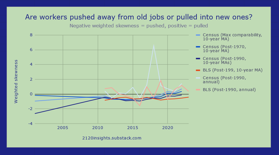
Other than in 2018 though, we see broad agreement across Census and BLS data that the strongest changes are coming from growing occupations rather than declining ones, pushing the skewness into new positive territory. It should be no surprise here that the Great Resignation of 2022, in which many workers left their old jobs for greener pastures elsewhere, was one of the most positive years on record for growing occupations driving more change than declining ones.
The smaller sample sizes of the Current Population Survey mean that month-to-month data even for larger occupations like Customer Service Representatives can be quite noisy:

It’s not unusual for employment to move by 2-3% in a month, which would be significant if sustained, but hard to determine a trend from one month of data alone. The larger occupational categories tracked by FRED might be broad enough to avoid this sort of noise, but the number of smaller occupations contained in the broader ones adds noise of its own.
(Thanks again GPT-4o for the quick and easy chart!)
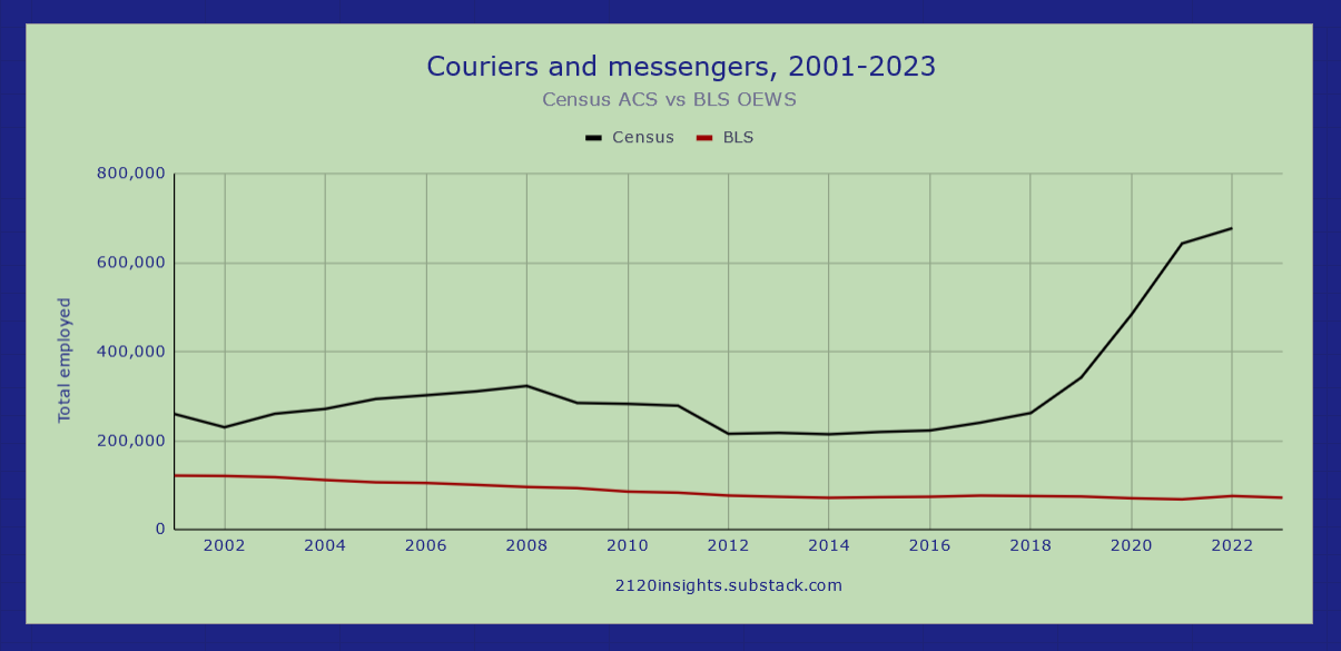
The growth of “Couriers and messengers” in Census data lines up quite well with interest in Doordash. But BLS data actually shows this occupation as in decline! This is likely due to its surveying of established businesses rather than independent contractors like Doordash delivery workers. This chart captures the strengths and weaknesses of both datasets: BLS data is more timely, but Census data is often more comprehensive (though workers in some areas may not identify their occupations as precisely as their employer would):
A note that this high-level chart is based on the “Max comparability” categories I detailed in the above footnote here. A further point of clarification on these: while every “Post-1990” occupation has no more than one “1970 broad” parent and one “Max comparability” grandparent, the relationship between each of these occupations and higher level designations that group multiple them together into larger categories is different.
Similar to the BLS Standard Occupational Classification (SOC), there are three levels of higher-level designations that occupations can fit under. From broadest to narrowest, they are:
Functional major category
Functional minor category
Functional broad occupation
Unlike the BLS SOC, not every occupation is assigned to a “Functional broad occupation”. Sometimes, the “Functional minor category” goes deep enough such that a third level category would be superfluous and just repeat the name of the occupation.
I also do add the “functional” qualifier to each of these categories because while they sometimes line up with the BLS designation, I have often made some changes, including:
Shifting BLS categorizations down a level to have fewer top-level categories
Shifting BLS categorizations up a level to highlight a particular category as more distinct
Allowing for supervisory and managerial occupations to be flexibly categorized as either part of the “Management, business & financial” major category, or as part of the category of worker who they are in charge of supervising
Creating a new category that I think adds value for comparative analysis
Shifting occupations to a category that is different from how it is categorized in BLS’ system for some other reason
Minor name changes
Aside from these differences from BLS categories, another key difference to be aware of is that the “1970 broad” and “Post-1990” children of a “Max comparability” occupation may belong to a completely different category from their parent. It is often the case that as occupations became more specifically defined over time, these realignments were necessary.
For example, the “Supervisors, managers, and executives” max comparability occupation belongs to the “Management, business & financial” major category. But “Supervisors of transportation and material moving workers” is split out from this as its own “1970 broad” occupation after 1970, and going forward, this occupation can be flexibly categorized as part of the “Transportation & moving” major category. This is the case for many management occupations, which is why looking at the same chart on an unadjusted basis, which looks how each level of occupation (Max comparability, 1970 broad, and Post-1990) side-by-side and without any transfer adjustments will show such big jumps in the key years of 1970 and 1990.

However, looking at the same chart strictly on a max comparability basis, even with no adjustments for transfer error (explained further below in the above footnote) doesn’t show as significant of changes. This is because on this basis, 1970 broad and later occupations such as “Supervisors of transportation and material moving workers” are still considered to be a part of “Supervisors, managers, and executives” and the higher level categories it belongs to: